LineaPy Internals

This document describes some of the high level code layout and implementation decisions.

What is a LineaPy Graph?

In LineaPy, we create a graph as we execute Python code, of every function that was called and its dependencies. We use this graph to do “program slicing,” meaning that we can understand all the code that is required to reproduce some value in your program.

As well as the program graph, we also store some information about how things were executed and the source code the graph was derived from.

We persist our graph structure to SQL (currently SQLite) using SQAlchemy, an ORM. The lineapy.data.types file stores the graph nodes and the lineapy.db.relational file stores the SQLAlchemy wrappers.

TODO: Visual of SQL table relationships

We have 6 different types of nodes in our graph currently. They all have an ID, and then have different attributes to describe their behavior. Each node conceptually has some “value” at runtime, so that when a node refers to another node, it can refer to its value.

Example:

This is an example file that when traced will make all six nodes:

import lineapy
from math import inf

x = [inf]
for i in range(10):
   x.append(i)

res = str(i + len(x))

These are the nodes that would be created from tracing this code (note that some attributes, like the session ID and source code references have been elided in the interest of transparency. The IDs are also UUIDs normally, but I have given them names for readability):

# The import node represents importing some module, in this case `math`.
ImportNode(
   id='math',
   name='math',
)

# A lookup node is similar to an import, but it looks up some name of a function
# from the builtins, in this case `getattr`
LookupNode(
   id='getattr',
   name='getattr'
)
# The literal node represents a literal primitive python value, like strings, ints,
# floats, etc. In this case it is the string "inf"
LiteralNode(
   id='inf_str',
   value='inf'
)
# When we import something from a module, this is translated as an import
# followed by a getattr call. This is represented by a CallNode, which
# represents calling some function with some arguments.
# In this case it gets the `inf` attribute from the `math` module.
CallNode(
   id='inf',
   function_id='getattr',
   positional_args=['math', 'inf_str']
)
# We have our own internal functions, all prefixed with `l_` that we use
# to implement certain python behavior. l_list takes a number of arguments
# and makes a list out of them. You might ask, why don't we just use the builtin
# `list`? Well that takes in some iterable as it's first argument.
# Another way to look at `l_list` is a function equivalent of the built in
# `[]` syntax.
LookupNode(
   id='l_list',
   name='l_list'
)
# We then finally are able to create `x` by calling l_list with infinity
CallNode(
   id='x',
   function_id='l_list',
   positional_args=['inf']
)

# Now we have a for loop. We currently "black box" this, treating it as a string
# which we end up `exec` through `l_exec_statement`
LiteralNode(
   id='loop_str',
   value='for i in range(10):\n    x.append(i)'
)
# We use our builtin `l_exec_statement` to compile and execute this code
LookupNode(
   id='l_exec_statement',
   value='l_exec_statement'
)
# Now we can actually call this string. Also notice that we pass in `x`
# as a dependency of this node, as a "global read" meaning that this node
# reads the global `x` we defined, for the node with id `x`.
CallNode(
   id='loop',
   function_id='l_exec_statement',
   positional_args=['loop_str'],
   global_reads={"x": "x"}
)
# Executing this loop creates a "mutate node" for value of x,
# meaning that any later references to x should refer to this mutate node,
# so that the code that mutated it, the loop, is also included implicitly
# as a dependency
MutateNode(
   id='x_mutated',
   source_id='x'
   call_id='loop'
)
# Executing this loop actually also sets the global `i`. We represent this
# with a GlobalNode, representing the global variable set by some call (we'll
# talk about how we detect the setting later):
GlobalNode(
   id='i_global',
   name='i',
   call_id='loop'
)

# Now when computing the result, we can point to this global node `i_global`
# as our input, as well as the mutate node
LookupNode(
   id='len',
   value='len'
)
CallNode(
   id='len_x',
   function_id='len',
   positional_args=['x_mutated'],
)
LookupNode(
   id='add',
   value='add'
)
CallNode(
   id='added',
   function_id='add',
   positional_args=['i_global', 'len_x'],
)
LookupNode(
   id='str',
   value='str'
)
CallNode(
   id='res',
   function_id='str',
   positional_args=['added'],
)

TODO: add visual of this in markdown with:

import lineapy

artifact = lineapy.save(res, "res")
artifact.visualize()

Creating Graphs

One main part of the codebase involves creating a graph from Python code.

We create this graph at runtime as we execute the Python code. We start with the AST of the Python and visit that as we turn it into a graph.

That goes through a number of steps, which we outline below, from outside in:

1. Entrypoint

We currently support two ways to start tracing from LineaPy. The CLI, which is used to trace Python scripts, and our Jupyter integration which is used in Jupyter Notebooks and IPython. Both of them go from source, to AST, to a graph.

CLI

In lineapy.cli.cli we support running a Python file from the CLI. That can produce some output, such as (1) printing out sliced code/graph, and (2) optionally to airflow file.

Exceptions

We also call set_custom_excepthook which is used to override Python’s sys.excepthook so that if an exception is raised from executing user’s code then we ignore all the frames added by lineapy (see “Exception handling” later in the doc).

Jupyter / IPython

We also supporting tracing using IPython (and so by proxy, Jupyter).

This is implemented in the lineapy.editors.ipython file. That class provides three main entry points:

1. start(): Starts tracing by adding a function to input_transformers_post which takes in a list of strings of the cell contents, and returns a list of strings which are executed by IPython.

2. stop(): Stops the tracing, removing this function from the input_transformers_post.

3. visualize(): output a visual of the current state of the graph.

In our input transformer, we save the code from the cell in a global and return the same lines from every cell, which call out to a function in the ipython module, _end_cell, which looks at the lines of code, transforms them through LineaPy, and optionally returns a value if one should be “returned” from the cell (i.e. if the last line is an expression that does not end with a ‘;’).

Exceptions

IPython does not use sys.excepthook so we have to take a different approach for handling exceptions in Jupyter. Instead, we set override the _get_exc_info method on the IPython shell, to have the same effect.

2. Parsing the AST

Once we have initialized lineapy with the user’s code, we traverse that through the python AST using a visitor defined in lineapy.transformer.node_transformer.

As we traverse the AST, we create nodes for each piece of it.

3. Creating nodes

This NodeTransformer relies on an lineapy.instrumentation.tracer.Tracer to actually create the nodes.

The general process to create a node is:

1. Create new instance of some Node subclass defined in types.py, giving it a new UUID.

2. Then in process_node pass the newly created node to the Executor to execute it, and return any “side effects” that happen

3. We react to those side effects, by potentially adding more nodes to the graph (which goes through step 1 one more time).

4. Write this node to the database.

We go into these side effects lower down, since they pertain to multiple layers.

4. Executing nodes

As mentioned above, the Tracer passes on the responsibility of executing the node to the lineapy.execution.executor.Executor. This is responsible for keeping a mapping of each node and its value after being executed.

It returns a number of “side effects” which say things like “Node xxx was modified” that the tracer can then handle. These are created based on the inspect_function’s side effects that are described below.

5. Determine function side effects

When we try to execute a CallNode, we need to know things like “does this modify any of its arguments?” to understand how it affects the graph.

This reasoning is implemented in lineapy.execution.inspect_function which is basically one big switch statement, that understands certain Python functions. If some function is not being sliced properly, it is likely due to it being missing from this file.

This also returns a list of “side effects,” which bubble up to the Executor. However, unlike the side effects returned from the executor, which refer to things by their node ID, in the inspect_function, the side effects instead refer to which arg/kwargs/value was modified. So it would say instead “The first arg was modified”.

This is to keep the inspect_function from having to know anything about nodes, and instead just about describing the side effects given some Python function call and values.

Reading graphs

After we have created a graph, we can perform a number of operations on it.

Many of these use the lineapy.data.graph object which represents a collection of nodes. It can sort them topologically and by line number, meaning that any node will come after its parents, and all nodes with line numbers will be sorted by those as well.

Note: It currently also include the session context, but we don’t really use this from the graph. We could remove this

Re-execution (steps 4-5)

We can re-execute a graph to re-run the Python function calls that were saved in it.

We keep the executor separate from the tracer, in order to facilitate this, so that we only need the Executor for re-execution, using the execute_graph method, which simply iterates through a number of nodes and executes each of them.

This is currently tested in our end to end tests, by re-executing every graph, but it is not currently exposed to the user.

Slicing

One common use of a graph is to “slice it”, meaning removing the nodes that are not ancestors of some input nodes.

We can use this then to output a “clean up” source code, where any lines that are not required to reproduce some result are removed. What this means is that the graph structure needs to represent program dependence, which is why some of our more complicated analysis are required.

This is implemented in lineapy.graph_reader.program_slice.

Visualizing

We currently supporting visualizing a graph using Graphviz for debugging and teaching purposes. This is implemented in the lineapy.visualizer directory with three main files:

1. lineapy.visualizer: Provides a Visualizer object which is the publicly exposed interface for visualizing a graph. In supports creating it for a number of different scenarios, each with their own configurations set. For example, we want to show more detail in our testing than in our public API. The visualizer also optionally supports taking a Tracer object, along with the required Graph object, to show more details that are present in that object, like the variable assignments. However, this is not always available, like when visualizing only a certain artifact, which can happen during re-execution, so the tracer is unavailable. It also supports a number of ways to viewing the visualization, like as SVG, PDF, or as Jupyter Output.

2. lineapy.visualizer.graphviz: This files manages actually creating the graphviz source using the Graphviz library. It renders each edge and node, and also renders a legend.

3. lineapy.visualizer.visual_graph.to_visual_graph(): This takes in the Graph and (optional) Tracer and returns a list of nodes and edges in a form that is closer to how Graphviz works. The goal of having this extra abstraction layer, as opposed to just emitting graphviz directly, is ensure a logically consistent rendering. It is similar to the MVC paradigm, or like React’s components. This would be equivalent to the props, where as the graphviz file is equivalent to taking those props and then rendering them.

Whenever a new node type is added, or any is modified, the graphviz and visual_graph files should be updated to handle it.

Outputting to airflow

On top of just slicing the code, we also support creating an Airflow DAG out of the resulting code. This is currently implemented through string templating in lineapy.plugins.airflow to create a file that airflow can understand.

All of the code is currently saved in one PythonOperator.

This is exposed to users in two ways:

1. In the cli through the –export-slice-to-airflow-dag flag, which will save the resulting DAG to the current directory.

2. In our API (usable in a script or in Jupyter) through the to_airflow method on a saved artifact. This is implemented in lineapy.graph_reader.apis. Instead of saving to the current directory, this tries to find Airflow’s DAGs folder, by looking at the AIRFLOW_HOME environment variable and saving it in there, so it is picked up by Airflow automatically.

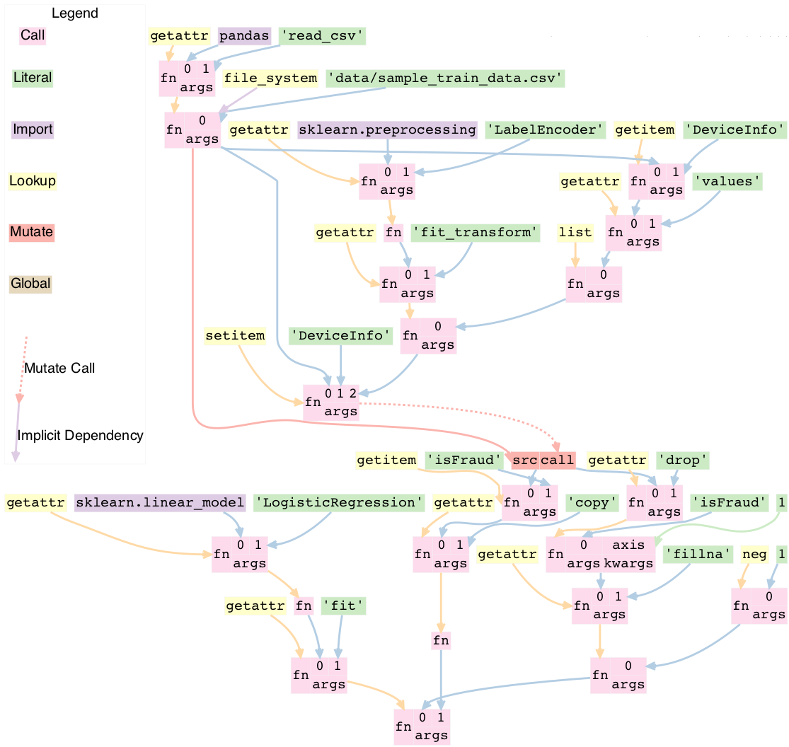
Put it all together

import pandas as pd
from sklearn.linear_model import LogisticRegression
from sklearn.preprocessing import LabelEncoder

train = pd.read_csv("data/sample_train_data.csv")

train['DeviceInfo'] = LabelEncoder().fit_transform(list(train['DeviceInfo'].values))

y = train['isFraud'].copy()

train = train.drop('isFraud', axis=1)
train = train.fillna(-1)

regression_model = LogisticRegression().fit(train, y)

Cross cutting concerns

Code Analysis (steps 3-5)

There are also a number of code analysis pieces that span the tracer-executor-inspect function, which we describe here.

Python Globals

The first is the ability to track what Python globals are set at any time.

For example in the code a = 1nb = a + 1 we have to know what the values a and b are at any given time. We can’t simply keep a values mapping as Python does because we also need to know the Node of each variable, not just it’s value, so we can stitch them together into the graph.

We currently keep this mapping in the Tracer. By the time it has been saved to the DB, the variable analysis has been erased. So the executor also has no knowledge of the variables.

The only exception to this is when dealing with execs and black boxes, which we touch on below.

Note: This is currently a problem for expressions like a = b which are entirely erased. This is fine for re-execution, but for slicing, this line is then omitted in the slice. We might want to re-consider this choice and instead have some way to persist the variables in the graph, possibly with some form of Assign and Load nodes.

Mutations and views

Since Python is not a pure functional language, many operations will mutate their arguments. Not only that, since objects often store references to one another internally, mutating one object can therefore mutate other objects as well.

For example, in this code:

x = []
y = [x]
y[0].append(1)

if we try to slice on either x or y, we will need to include all three lines to get back the proper result for either variable. We represent this internally with two concepts:

1. We say a node is “mutated” if the semantics of the Python value it refers to has changed. A mutation is often the result of calling some function. Another way to think about this is that if calling some function would change how downstream usage or evaluation of a node behaves, then we can say that function call mutated that node.

2. We saw two nodes are “views” of one another if mutating one node could mutate the other node. Since it’s better to be conservative in slicing, we assume it does. We currently treat views as a bidirectional relationship, meaning we assume if mutating a could affect b, then the opposite is also true.

Once we start with these two concepts a few things fall out:

1. We need to know during each function call what nodes are directly mutated.

2. We need a way in the graph to have any later references to a node that was mutated implicitly also depend on the call node that mutated it, so that this will be included in the slice.

3. We need to know during each call what views were added.

4. We need to know when a node is mutated, what other nodes are views of it.

For #1, this starts in inspect_function.py. If we know calling a function will mutate a value, we return a MutatedValue with a pointer to that value as one of the side effects. Then in executor.py we “resolve” that to a MutatedNode value, since we now know the node ID of the mutated value, not just if it was say the first argument.

For #2, we add a new node type, a MutateNode, which points both to its original value and the call node which created it. Then in the Executor when we see we have a MutatedNode side effect we know to make a new MutateNode (note the difference, one is a side effect saying a node was mutated, the other is a new node type that represents the result of this mutation). It also updates a mapping that points from each source node to its mutate node, so that when we then go to lookup a node, we point to the mutate node, instead of the source. This mapping and the logic to update it is kept in lineapy.instrumentation.mutation_tracker.

For #3, similar to #1, inspect_function returns a ViewOfValues, which is transformed into a ViewOfNodes in the Executor.

And for #4, when we see this side effect in the Tracer, we update our internal data structure keeping track of all views in mutation_tracker.py. And when we see that a node is mutated, we look into this data structure to also see what other nodes should be mutated.

Execs and “black boxes”

Currently, we don’t try to understand any builtin Python control flow or anything besides expressions. So for constructs like function definitions, loops, if statements, while statements we treat them as “black boxes”.

This mostly works fine, but we still need to know what global variables a black box wrote to and which it read from, in order to add it properly to the graph.

The life of a black box node goes through a number of stages:

1. In the node_transformer when we see the AST statements that correspond to things like for loops, we tell the Tracer to add a a literal node for the string, and then a CallNode which execs the string. We differentiate between exec-ing a “statement” versus an “expression”, since an expression will return some value, while a statement does not.

2. The functions we use to do the exec are defined in lineapy.utils.lineabuiltins, lineapy.utils.lineabuiltins.l_exec_statement() and lineapy.utils.lineabuiltins.l_exec_expr(). Along with actually calling exec, they set up the source code context, so that exceptions raised in code that is `exec`ed has the proper traceback and also make sure to use it uses the correct globals.

3. Before this call node is executed, we set the lineapy.execution.context.ExecutionContext, which is a global storing the current node and executor being called. This allows us to use the current binding of the global variables in the l_exec_expr and l_exec_statement functions.

4. When we are tracing code, we initialize the globals with all globals we have traced so far. However, when re-executing, we look at the global_reads dictionary on the CallNode to see what variables are read and what nodes they correspond to. On to how that is set below…

5. After calling the function, the globals in the context now contains all the new globals that were set or re-assigned in the exec. We look at this dict, and check which nodes have changed to see what globals have been written to. To see what globals were read, we use a dict subclass called lineapy.execution.globals_dict.GlobalsDict which keeps track of all __getitem__ calls.

6. We store all values that were accessed under the global_reads dictionary on the CallNode, so when we slice on this node, it will include those dependencies, and when we re-execute it, it will know which globals to set.

7. For each new global that was set, or updated, we create a GlobalNode, which points to the call node that created the global, as well as the variable name. Also in the Executor we add an item to the internal mapping _node_to_globals which keeps track of all the globals returned by each node. Then, later on, if a node refers to this GlobalNode, it can look up in this mapping to find the value that was set in the globals when executing that node.

One subtle case to consider is that globals are not only read and wrote during the execution of our exec nodes, but also potentially during execution of functions that were defined in them, or any other function that modifies or sets a global.

For example:

a = 1
def inc_i():
   global a
   a += 1

lineapy.save(a, "first")
inc_i()
lineapy.save(a, "second")

In this case, we will call l_exec_statement with the body of text of inc_i and this will create a GlobalNode for inc_i that points to that CallNode.

Then, calling it will create a CallNode that will use that global node of inc_i as the function, set global_reads to map “a” to the original a literal node, and create a new GlobalNode for the new value of a.

Another way of thinking about the GlobalNode is a way to represent things that were “returned” by a function call implicitly. Instead of making a new node, we could change how we think about nodes, that instead of having one returned value, they have also have additional variables they set, and/or possibly multiple return values. This would make it more symmetrical to how we think about function inputs.

In a similar manner, we could remove `MutateNode`s and represent them instead in our function inputs.

However, this would require changing all our references to not only say “we depend on node XXX” but also what part of it we depend on like “we depend on the return value of node XXX” or “we depend on the global x set by node XXX” or “we depend on the mutated value of node YYY set by calling XXX.”

For now though, we do have this asymmetry, where the global inputs show up as the global_reads property on the CallNode and the global outputs show up as separate `GlobalNode`s.

External side effects

Another example of implicit state, besides global variables, are external side effects, like writing to a file or reading from SQL. This shows up in two types of use cases. The first, is when you have some node that depends on another implicitly based on a side effect, like this:

write_file("hello", 'text')
x = read_file("hello")

If we slice on x we probably also want to include the write file, since this needs to be executed before we read it.

A similar use case comes up if the result of our script is writing to a file, and we want to preserve this effect, to say create an airflow job that writes to a file. We can write this like:

write_file("hello", 'text')
lineapy.save(lineapy.file_system, "wrote file")

We can think about these use cases under this framework:

1. We have an implicitly defined node for each type of side effect, like touching the file system or writing to S3.

2. Whenever we have a node which writes a side effect, we create a mutate node for that implicitly defined node.

3. Whenever we have a node that depends on the state of that side effect, we add that node as an implicit dependency.

4. Whenever we manually refer to that implicit node, as in lineapy.utils.lineabuiltins.file_system we have this also have an implicit dependency on the most recent version of that node.

Currently we only support the broad categories of side effects, but we can expand this to have more fine grained support in the future, like writing to a particular file.

We implement the following framework by:

1. We create a global for file_system and db in lineapy.utils.lineabuiltins. Both of these are instances of ExternalState, a class defined in that file. This lets them be accessed through a LookupNode.

2. We can bubble this up from the inspect_function.py by passing an instance of ExternalState in as an arg for MutatedValue or ViewOfValues to represent that a function is mutates that state or is a view of it (subsequent mutates will mutate that state).

3. That is bubbled up through the Executor, so that it’s MutateNode can also point to a ExternalState instead of just a node ID.

4. At the Tracer level, when we are looking at side effect, if it refers to an ExternalState, we make a lookup node for it.

5. In the Executor as we are processing this LookupNode, in execute_node, we see that it returns an ExternalState (this happens in execute_node) and we check to see if we have already created a node. If so we add a ImplicitDependencyNode side effect which points to the existing node.

6. Then when this LookupNode’s side effects are processed in the Tracer, if we find an ImplicitDependencyNode we add this to the list of implicit_dependencies of that node.

Also, for the second use case, where we do the getattr on lineapy to return file_system, this executes steps 5-6, to also add an implicit dependency on the previously defined value.

Bound self

One other cross cutting concern is that many methods modify the “self” they are bound to. However, this is not really an argument, as far as we are concerned, but a property of the function itself.

For example this code:

`python l = [] l.append(1) `

Is executed like this in LineaPy:

`python l = l_build_list() l_append = getattr(l, "append") l_append(1) `

So when l_append is called, the function is the bound method and only has one arg. So how can we track that calling it modifies the object it was bound to?

We do this by:

1. Having a special value BoundSelfOfFunction in inspect_function that refers to the object the function is a method from.

2. In the executor we keep a mapping of _node_to_bound_self which we update every time we see a getattr. In our case, this would be mapping the ID of l_append to the ID of l.

3. When we see the BoundSelfOfFunction in the Executor, we look up the ID of the node in this mapping, and use that as the ID to pass on to the Tracer.

We can see this being used in the code to deal with append in inspect_function:

if (
   isinstance(function, types.BuiltinMethodType)
   and function.__name__ == "append"
   and isinstance(function.__self__, list)
):
   # list.append(value)
   yield MutatedValue(BoundSelfOfFunction())
   if is_mutable(args[0]):
      yield ViewOfValues(BoundSelfOfFunction(), PositionalArg(0))
   return

This says that if the function is a method, it’s name is append, and its a method from list, then we mutated the self value, and if the input is a mutable value, we treat that as a view of the list. This is so that if we append something mutable, and we later mutate that, the list is mutated, and vice versa.

LineaPy API (step 4)

Although LineaPy does not require any annotations to trace your code, we do provide some functions that you can use to annotate it to tell us what is important and also to interact with LineaPy. These are defined in lineapy.api and returns objects defined in lineapy.graph_reader.apis.

Implementing these functions require us to break a key abstraction we have which is that executing code while tracing LineaPy should perform the same as while not tracing with LineaPy.

We need to break this, since these functions implicitly require us to know what database we are tracing with and also what nodes certain values point to, in the case of save.

You might notice this abstraction is also broken in the l_exec_statement function, we mentioned above, since it needs to know the source code of the string as well as the global variables defined.

_Writing this, I realize that we might not need the context for the l_exec functions, since we could pass the source code path and line number as explicit args, and get access to the globals with globals(). Some future work could be to refactor that to make it explicit and remove the need to use get_context()._

We break this abstraction by having the executor set up a global context, using set_context before it calls any nodes, and providing the get_context function to retrieve it. These are both defined in lineapy.execution.context.

This lets our API functions access the current node being executed, as well as the current DB.

Exception handling (steps 1 and 4)

We do two special things to change how exceptions are handled:

1. In step 1: Remove the frames we add in LineaPy off of the stack to show a user their original exception. We do this by raising a lineapy.exceptions.user_exception.UserException which contains the original exception that was raised. Then in Step 1 above (either in the CLI or Jupyter), we see if the exception raised was a UserException and if so we just use the inner exception.

2. In step 4: Change the top frame to reflect the source code position of the original code. For example, if we see 1 + 2, this is transformed to us calling operator.add(1, 2). We don’t want to point them to where we do this call, but instead point to the source code which originated it. We do this by removing the top frame, and adding back a fake frame with the proper source code position. Then when python prints the exception, it will look the same. This is done in lineapy.exceptions.user_exception and the fake frame creation in lineapy.exceptions.create_frame.